关于联邦学习
-
联邦学习出现的背景
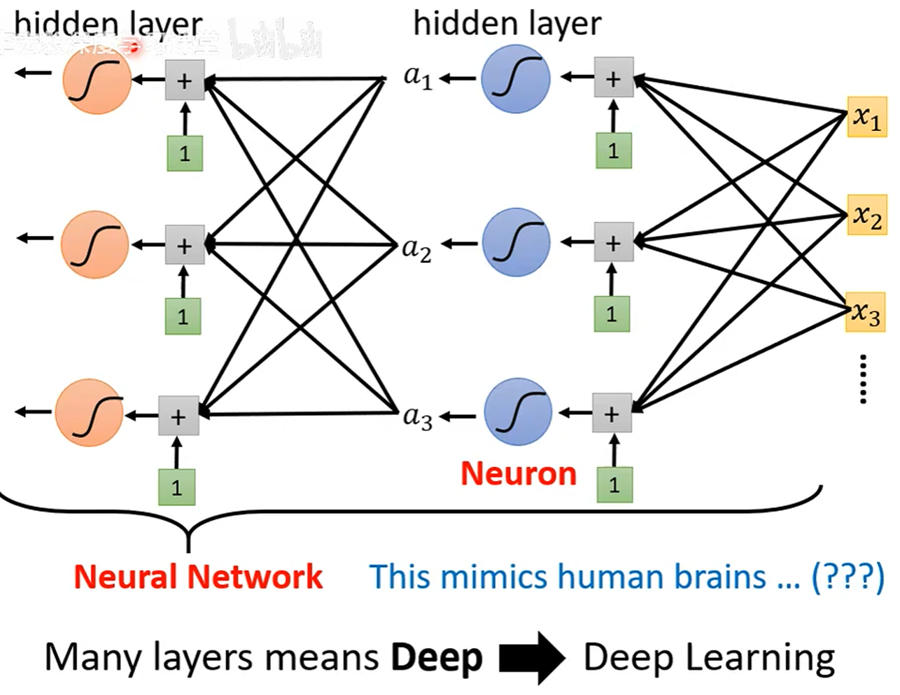
- 移动设备上有大量数据可用来机器学习,但是这些数据往往是涉及隐私的
- 传统的分布式AI训练是IID的(每个设备上的数据都是均匀的),但是在移动设备上,根据用户习惯的不同,不同设备间的数据存在显著差异
- 移动设备上的计算成本相对较低,而通信成本相对较高
-
联邦学习的机制
- 服务器初始化一个模型,分发给一定比例的移动端,这些模型的初始位置是相同的
- 客户端接收到模型之后,用本地的数据进行训练,上传更新后的模型数据而不是本地的数据集
- 而后,服务端按照每台移动设备处理的样本数来加权计算梯度下降,更新模型的参数
- 其中,需要调整的参数:C(本轮参与训练的客户端比例),E(本地的epoch数量),B(本地批次大小),η(学习率)
-
FedSGD和FedAvg
- FedSGD:全部客户端在本地进行一次训练后,将结果返回服务器
- FedAvg:部分客户端在本地进行多轮训练,将多轮训练后的结果返回给服务器
-
特性 FedSGD FedAvg 本地计算量 少 多 通信轮数 多 少 每轮通信成本 低 高 取舍关系 用通信换计算 用计算换通信 本地更新 一次梯度计算 E个epoch的本地训练 参数B B=∞(整个本地数据集作为一个batch) B可调(多次训练) 参数E E=1(只进行一次训练) E≥1
实验复现
-
环境配置
-
Python 3.13
- Matplotlib 3.10.7
-
Conda 25.9.1
- PyTorch 2.9.1+cu128
- TorchVision 0.24.1+cu128
- Numpy 2.3.3
-
-
数据集处理(data_utils.py)
-
导入依赖
import numpy as np import torchvision import torchvision.transforms as transforms-
从MNIST准备数据
# 从MNIST准备数据.其中,num_clients代表客户端数量,布尔值iid表示是否按照IID方式划分 def prepare_mnist_data(num_clients=100, iid=True): # 数据预处理 transform = transforms.Compose([ # 将输入数据转化为PyTorch张量 # 转换像素值,避免梯度爆炸 transforms.ToTensor(), #将张量标准化(将数据调整为正态分布) transforms.Normalize((0.1307,), (0.3081,)) ]) #下载MNIST数据集:将训练集和测试集从互联网下载到./data目录,预处理方式为上面的Compose transform trainset = torchvision.datasets.MNIST(root='./data', train=True,download=True, transform=transform) testset = torchvision.datasets.MNIST(root='./data', train=False,download=True, transform=transform) # 划分数据到客户端:返回划分后的结果和处理后的完整数据集 if iid: #按照IID划分 return split_iid(trainset, num_clients), trainset, testset else: #不按照IID划分 return split_non_iid(trainset, num_clients), trainset, testset-
按照IID划分数据
#按照IID划分:打乱后随机分配,理想化模型 def split_iid(dataset, num_clients): #计算每个客户端应该分到的数据量(向下取整的整除) num_items = len(dataset) // num_clients #创建记录客户端与对应值的字典,键为客户端ID,值为一个集合,其中存储客户端拥有的数据索引 dict_clients = {} #使用range()创建一个列表,包含整个数据集的索引 all_idxs = list(range(len(dataset))) #将all_idxs打乱(使用numpy中的random模块) np.random.shuffle(all_idxs) #循环遍历客户端,为其分配数据(将乱序的all_idxs切片) for i in range(num_clients): dict_clients[i] = set(all_idxs[i * num_items:(i + 1) * num_items]) #返回客户端与数据索引的对应关系 return dict_clients-
按照NonIID划分数据
#按照NonIID划分,数据不均匀,更接近真实情况 def split_non_iid(dataset, num_clients, shards_per_client=2): #1.按标签排序 #创建索引数组idxs,包含了所有数据的索引 idxs = np.arange(len(dataset)) #提取数据集中所有样本的标签(返回一个由列表得出的numpy数组) labels = np.array([dataset[i][1] for i in range(len(dataset))]) #垂直堆叠索引数组和标签数组,成为一个二维数组:第一个元素是存储有序idxs的np数组,第二个元素是存储对应标签的np数组 idxs_labels = np.vstack((idxs, labels)) #idxs_labels[1, :].argsort()返回idxs_labels[1, :]的从小到大排序(索引位置) #外层函数排列整个矩阵的位置,最后返回一个按照标签值排序的二维数组idxs idxs_labels = idxs_labels[:, idxs_labels[1, :].argsort()] #从排序好的矩阵中提取索引数组(按照标签排列) idxs = idxs_labels[0, :] #这样,连续索引的数据相似度很高,符合NonIID的情况 #2.创建分片 #shards_per_client表示每个客户端得到的分片数量,值越小,客户端的数据越同质,Non-IID的程度越高 total_shards = num_clients * shards_per_client #按照总分片数来对数据切片(切片原理和IID类似) shard_size = len(dataset) // total_shards shard_idxs = [set(idxs[i * shard_size:(i + 1) * shard_size].astype(int)) for i in range(total_shards)] #3.分配分片给客户端 #与IID模式下的分片类似 dict_clients = {} shards = np.arange(total_shards) np.random.shuffle(shards) #以分片为单位给客户端分配数据 for i in range(num_clients): #selected_shards是shards的切片.表示当前客户端被分配的分片索引 selected_shards = shards[i * shards_per_client:(i + 1) * shards_per_client] #给每个客户端初始化一个新的集合,其中dict_clients的键为客户端索引,值为一个集合,存储分片的索引 dict_clients[i] = set() #把分片索引添加到dict_clients的值中 for shard in selected_shards: dict_clients[i] = dict_clients[i].union(shard_idxs[shard]) return dict_clients -
-
模型构建(models.py)
-
导入依赖
import torch.nn as nn import torch.nn.functional as F-
MNIST 2NN(两层MLP)
class MLP(nn.Module): #所有PyTorch模型都必须继承nn.Module #初始化模型网络层和参数 def __init__(self): #父类构造函数来自继承的nn.Module,保证nn.Module被正常初始化 super(MLP, self).__init__() #定义全连接层:参数分别是输入维度(展平后的图像大小)和输出维度 self.fc1 = nn.Linear(784, 200) #第二层接收第一层的输入,并且输出二百维 self.fc2 = nn.Linear(200, 200) #第三层输出十位,即十个数字的识别 self.fc3 = nn.Linear(200, 10) #定义前向传播函数,x是输入张量 def forward(self, x): #view()函数改变张量形状但是不改变数据,-1通常是batch_size,784表示784个维度 x = x.view(-1, 784) #将x通过两次relu前向传播 x = F.relu(self.fc1(x)) x = F.relu(self.fc2(x)) x = self.fc3(x) return F.log_softmax(x, dim=1)-
MNIST CNN(CNN模型)
class CNN(nn.Module): def __init__(self): super(CNN, self).__init__() #定义卷积层:输入通道数,输出通道数,卷积核大小,padding(边缘填充像素) self.conv1 = nn.Conv2d(1, 32, 5, padding=2) self.conv2 = nn.Conv2d(32, 64, 5, padding=2) self.fc1 = nn.Linear(7 * 7 * 64, 512) self.fc2 = nn.Linear(512, 10) def forward(self, x): x = F.relu(self.conv1(x)) x = F.max_pool2d(x, 2) x = F.relu(self.conv2(x)) x = F.max_pool2d(x, 2) x = x.view(-1, 7 * 7 * 64) x = F.relu(self.fc1(x)) x = self.fc2(x) return F.log_softmax(x, dim=1) -
-
FedAvg算法实现(fedavg_algorithm.py)
-
导入依赖
import torch import torch.nn.functional as F import torch.optim as optim from torch.utils.data import DataLoader, Subset import numpy as np import copy-
初始化FedAvg类
class FedAvg: def __init__(self, model, train_dataset, test_dataset, client_data_dict, device=None): # 设置设备:优先使用cuda,显卡不可用时使用cpu if device is None: self.device = torch.device("cuda" if torch.cuda.is_available() else "cpu") else: self.device = device print(f"使用设备: {self.device}") # 将模型移动到设备 self.global_model = model.to(self.device) #将传入的参数赋值给类本地的参数 self.train_dataset = train_dataset self.test_dataset = test_dataset self.client_data_dict = client_data_dict #获取客户端数量 self.num_clients = len(client_data_dict)-
实现客户端本地的更新
#实现客户端本地的更新,其中client_id是客户端索引,E是本地训练的epoch数,B表示BatchSize,lr表示LearningRate def client_update(self, client_id, global_model, E, B, lr): #选用深拷贝,而不是直接引用,保证每个客户端都是独立的模型,互不干扰 local_model = copy.deepcopy(global_model) #将模型设置为训练模式:启用Dropout层,训练时随机失效神经元,防止过拟合,并开启梯度计算 local_model.train() #为客户端从完整数据集中抽取专属子集 client_data = Subset(self.train_dataset, list(self.client_data_dict[client_id])) #创建数据加载器:每批次数据有B个,每个epoch都打乱顺序训练 client_loader = DataLoader(client_data, batch_size=B, shuffle=True) #使用随机梯度下降优化器:local_model.parameters()代表模型参数,包含权重和偏置,lr是学习率,乘上微分来控制步长 optimizer = optim.SGD(local_model.parameters(), lr=lr) # 本地训练E个epoch for epoch in range(E): for batch_idx, (data, target) in enumerate(client_loader): # 将数据移动到设备,确保数据和模型在同一设备上(PyTorch要求所有计算在相同设备上进行) data, target = data.to(self.device), target.to(self.device) #清空梯度(PyTorch会累积梯度,清空来避免梯度叠加) optimizer.zero_grad() #前向传播,计算预测值 output = local_model(data) #计算Loss(输入模型预测和真实标签) loss = F.nll_loss(output, target) #反向传播,计算梯度 loss.backward() #更新模型参数(lr*梯度向量) optimizer.step() #返回本地模型的状态字典 return local_model.state_dict()-
评估模型性能
#评估模型性能 def evaluate(self, model, dataloader): #将模型设定为评估模式 model.eval() #初始化损失值和正确样本数的计数器 test_loss = 0 correct = 0 #下面的代码中不需要进行梯度运算,因为目的是评估而不是训练 with torch.no_grad(): #从数据加载器中获取数据 for data, target in dataloader: # 将数据移动到同一设备 data, target = data.to(self.device), target.to(self.device) #推理输出 output = model(data) #计算Loss并求和累加 test_loss += F.nll_loss(output, target, reduction='sum').item() #获取预测结果(找出概率最大的索引值) pred = output.argmax(dim=1, keepdim=True) #统计正确预测数量 correct += pred.eq(target.view_as(pred)).sum().item() #计算平均Loss test_loss /= len(dataloader.dataset) #计算准确率 accuracy = 100. * correct / len(dataloader.dataset) #返回损失和准确率 return test_loss, accuracy-
FedAvg训练过程
#FedAvg训练过程:C表示每轮选择的客户端比例,num_rounds表示通信轮数(总训练数),target_accuracy:目标准确率 def train(self, C, E, B, lr, num_rounds, target_accuracy=None): #创建数据加载器,shuffle:是否需要乱序 test_loader = DataLoader(self.test_dataset, batch_size=1000, shuffle=False) # 初始化记录结果:达到目标需要的轮数,准确率,通信轮数 rounds_to_target = None accuracy_history = [] communication_rounds = [] print(f"开始训练: C={C}, E={E}, B={B}, lr={lr}") for round_idx in range(1, num_rounds + 1): #计算每轮的客户端数量 m = max(int(C * self.num_clients), 1) #无放回抽样地随机选择客户端 selected_clients = np.random.choice(range(self.num_clients), m, replace=False) #初始化每个客户端的模型参数和数据大小 local_weights = [] client_sizes = [] #对每一个客户端进行训练 for client_id in selected_clients: #调用客户端本地更新函数,返回更新后的模型参数并记录,并使数据量++ local_weight = self.client_update(client_id, self.global_model, E, B, lr) local_weights.append(local_weight) client_sizes.append(len(self.client_data_dict[client_id])) # 服务器聚合(加权平均) total_size = sum(client_sizes) global_weights = copy.deepcopy(local_weights[0]) for key in global_weights.keys(): global_weights[key] *= client_sizes[0] / total_size for i in range(1, len(local_weights)): for key in global_weights.keys(): global_weights[key] += local_weights[i][key] * client_sizes[i] / total_size # 更新全局模型(以服务端聚合后的参数来更新全局模型) self.global_model.load_state_dict(global_weights) # 评估 test_loss, accuracy = self.evaluate(self.global_model, test_loader) accuracy_history.append(accuracy) communication_rounds.append(round_idx) if round_idx % 10 == 0: print(f'Round {round_idx}: Test Accuracy = {accuracy:.2f}%') # 检查是否达到目标精度 if target_accuracy and accuracy >= target_accuracy and rounds_to_target is None: rounds_to_target = round_idx print(f'达到目标精度 {target_accuracy}% 在 {round_idx} 轮') break return communication_rounds, accuracy_history, rounds_to_target -
-
实验配置(experiments.py)
-
导入依赖
import torch from data_utils import prepare_mnist_data from fedavg_algorithm import FedAvg from models import MLP, CNN-
判断设备
def run_experiments(): # 检查GPU可用性 device = torch.device("cuda" if torch.cuda.is_available() else "cpu") print(f"检测到设备: {device}") if torch.cuda.is_available(): print(f"GPU名称: {torch.cuda.get_device_name(0)}") print(f"GPU内存: {torch.cuda.get_device_properties(0).total_memory / 1024**3:.1f} GB")-
设置实验
configs = [ # (模型类型, 数据分布, C, E, B, 目标精度, 轮数) ('MLP', 'IID', 0.1, 1, 10, 90.0, 50), ('MLP', 'IID', 0.1, 5, 10, 90.0, 50), ('MLP', 'Non-IID', 0.1, 1, 10, 90.0, 50), ('MLP', 'Non-IID', 0.1, 5, 10, 90.0, 50), ('CNN', 'IID', 0.1, 1, 10, 95.0, 50), ('CNN', 'IID', 0.1, 5, 10, 95.0, 50), ]-
进行训练
results = {} for config in configs: model_type, data_dist, C, E, B, target_acc, num_rounds = config print(f"\n=== 实验配置: {model_type}-{data_dist}-C{C}-E{E}-B{B} ===") # 准备数据 client_data_dict, trainset, testset = prepare_mnist_data( num_clients=100, iid=(data_dist == 'IID') ) # 选择模型 if model_type == 'MLP': model = MLP() else: model = CNN() # 训练 - 传入device参数 fedavg = FedAvg(model, trainset, testset, client_data_dict, device=device) comm_rounds, acc_history, rounds_to_target = fedavg.train( C=C, E=E, B=B, lr=0.01, num_rounds=num_rounds, target_accuracy=target_acc ) # 保存结果 key = f"{model_type}_{data_dist}_C{C}_E{E}_B{B}" results[key] = { 'rounds_to_target': rounds_to_target, 'accuracy_history': acc_history, 'communication_rounds': comm_rounds } return results -
-
结果可视化(visualization.py)
-
导入依赖
import matplotlib.pyplot as plt import pickle-
设置字体
# 设置中文字体和正负号 plt.rcParams['font.sans-serif'] = ['SimHei', 'Microsoft YaHei', 'DejaVu Sans'] plt.rcParams['axes.unicode_minus'] = False-
绘制学习曲线
def plot_results(results): #绘制不同配置下的学习曲线 plt.figure(figsize=(15, 10)) # 为不同配置定义颜色和线型 colors = ['blue', 'red', 'green', 'orange', 'purple', 'brown'] line_styles = ['-', '--', '-.', ':'] # 按模型类型分组 mlp_results = {k: v for k, v in results.items() if 'MLP' in k} cnn_results = {k: v for k, v in results.items() if 'CNN' in k} # 绘制MLP结果 plt.subplot(2, 1, 1) for i, (config, result) in enumerate(mlp_results.items()): color = colors[i % len(colors)] linestyle = line_styles[i // len(colors) % len(line_styles)] rounds = result['communication_rounds'] accuracy = result['accuracy_history'] plt.plot(rounds, accuracy, color=color, linestyle=linestyle, linewidth=2, label=config) plt.title('MLP模型 - 测试准确率 vs 通信轮数') plt.xlabel('通信轮数') plt.ylabel('测试准确率 (%)') plt.legend() plt.grid(True) # 绘制CNN结果 plt.subplot(2, 1, 2) for i, (config, result) in enumerate(cnn_results.items()): color = colors[i % len(colors)] linestyle = line_styles[i // len(colors) % len(line_styles)] rounds = result['communication_rounds'] accuracy = result['accuracy_history'] plt.plot(rounds, accuracy, color=color, linestyle=linestyle, linewidth=2, label=config) plt.title('CNN模型 - 测试准确率 vs 通信轮数') plt.xlabel('通信轮数') plt.ylabel('测试准确率 (%)') plt.legend() plt.grid(True) plt.tight_layout() plt.savefig('fedavg_results.png', dpi=300, bbox_inches='tight') plt.show()-
分析FedAvg相比FedSGD的加速比
def analyze_speedup(results): #分析FedAvg相比FedSGD的加速比 print("\n=== 加速比分析 ===") # 基准:FedSGD (E=1, B=∞) baseline_configs = { 'MLP_IID': None, 'MLP_Non-IID': None, 'CNN_IID': None, 'CNN_Non-IID': None } # 找到基准配置的轮数 (E=1) for config, result in results.items(): if 'E1' in config: if 'MLP_IID' in config: baseline_configs['MLP_IID'] = result['rounds_to_target'] elif 'MLP_Non-IID' in config: baseline_configs['MLP_Non-IID'] = result['rounds_to_target'] elif 'CNN_IID' in config: baseline_configs['CNN_IID'] = result['rounds_to_target'] elif 'CNN_Non-IID' in config: baseline_configs['CNN_Non-IID'] = result['rounds_to_target'] # 计算加速比 speedup_table = [] for config, result in results.items(): if result['rounds_to_target'] is not None: if 'MLP_IID' in config and baseline_configs['MLP_IID']: speedup = baseline_configs['MLP_IID'] / result['rounds_to_target'] speedup_table.append((config, result['rounds_to_target'], speedup)) elif 'MLP_Non-IID' in config and baseline_configs['MLP_Non-IID']: speedup = baseline_configs['MLP_Non-IID'] / result['rounds_to_target'] speedup_table.append((config, result['rounds_to_target'], speedup)) elif 'CNN_IID' in config and baseline_configs['CNN_IID']: speedup = baseline_configs['CNN_IID'] / result['rounds_to_target'] speedup_table.append((config, result['rounds_to_target'], speedup)) elif 'CNN_Non-IID' in config and baseline_configs['CNN_Non-IID']: speedup = baseline_configs['CNN_Non-IID'] / result['rounds_to_target'] speedup_table.append((config, result['rounds_to_target'], speedup)) # 打印加速比表格 print("\n配置\t\t\t\t轮数\t加速比") print("-" * 50) for config, rounds, speedup in sorted(speedup_table, key=lambda x: x[2], reverse=True): print(f"{config:30} {rounds:4d} \t{speedup:5.1f}x") return speedup_table-
实验结果的保存与读取
def save_results(results, filename='fedavg_results.pkl'): #保存实验结果到文件 with open(filename, 'wb') as f: pickle.dump(results, f) print(f"结果已保存到 {filename}") def load_results(filename='fedavg_results.pkl'): #从文件加载实验结果 with open(filename, 'rb') as f: results = pickle.load(f) return results -
-
实验运行(main.py)
-
导入依赖
from experiments import run_experiments from visualization import plot_results, analyze_speedup, save_results-
主函数
def main(): print("开始联邦学习FedAvg算法复现实验") print("=" * 50) print("\n步骤1: 运行实验") results = run_experiments() print("\n步骤2: 可视化结果") plot_results(results) print("\n步骤3: 分析加速比...") analyze_speedup(results) print("\n步骤4: 保存结果...") save_results(results) print("\n实验完成!") if __name__ == "__main__": main() -
-
实验结果
开始联邦学习FedAvg算法复现实验
==================================================

步骤1: 运行实验
检测到设备: cuda
GPU名称: NVIDIA GeForce RTX 5060 Laptop GPU
GPU内存: 8.0 GB

=== 实验配置: MLP-IID-C0.1-E1-B10 ===
使用设备: cuda
开始训练: C=0.1, E=1, B=10, lr=0.01
达到目标精度 85.0% 在 5 轮

=== 实验配置: MLP-IID-C0.1-E5-B10 ===
使用设备: cuda
开始训练: C=0.1, E=5, B=10, lr=0.01
达到目标精度 85.0% 在 2 轮

=== 实验配置: MLP-Non-IID-C0.1-E1-B10 ===
使用设备: cuda
开始训练: C=0.1, E=1, B=10, lr=0.01
Round 10: Test Accuracy = 51.47%
Round 20: Test Accuracy = 70.68%
Round 30: Test Accuracy = 80.79%
达到目标精度 85.0% 在 39 轮

=== 实验配置: MLP-Non-IID-C0.1-E5-B10 ===
使用设备: cuda
开始训练: C=0.1, E=5, B=10, lr=0.01
Round 10: Test Accuracy = 77.70%
达到目标精度 85.0% 在 17 轮

=== 实验配置: CNN-IID-C0.1-E1-B10 ===
使用设备: cuda
开始训练: C=0.1, E=1, B=10, lr=0.01
Round 10: Test Accuracy = 94.77%
达到目标精度 95.0% 在 12 轮

=== 实验配置: CNN-IID-C0.1-E5-B10 ===
使用设备: cuda
开始训练: C=0.1, E=5, B=10, lr=0.01
达到目标精度 95.0% 在 3 轮

步骤2: 可视化结果

步骤3: 分析加速比...

=== 加速比分析 ===

配置                轮数  加速比
--------------------------------------------------
CNN_IID_C0.1_E5_B10               3     4.0x
MLP_IID_C0.1_E5_B10               2     2.5x
MLP_Non-IID_C0.1_E5_B10          17     2.3x
MLP_IID_C0.1_E1_B10               5     1.0x
MLP_Non-IID_C0.1_E1_B10          39     1.0x
CNN_IID_C0.1_E1_B10              12     1.0x

步骤4: 保存结果...
结果已保存到 fedavg_results.pkl

实验完成!

进程已结束,退出代码为 0
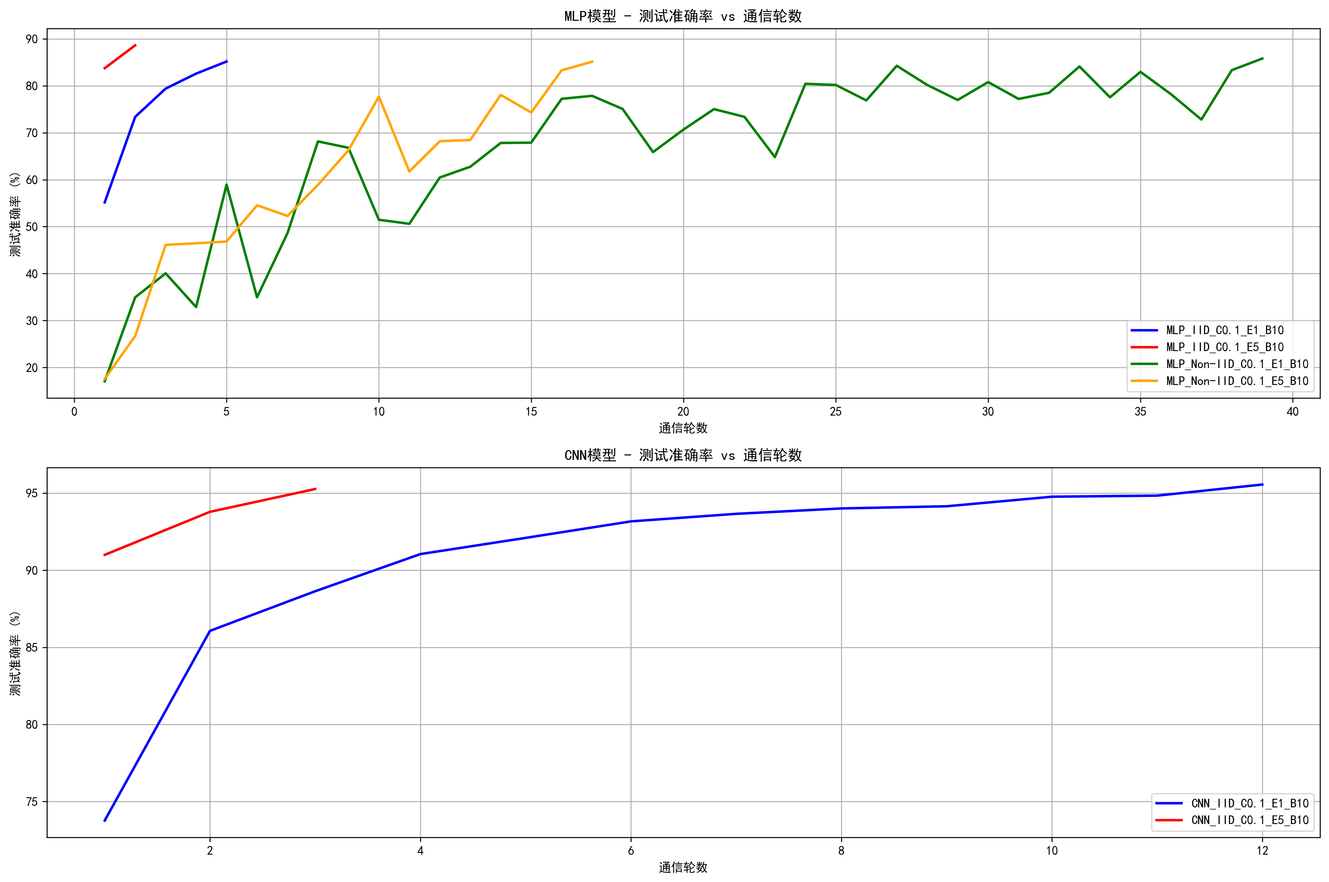
复现的结果很好: